60-1
% halbkugelkontur.m
z=zeros(41);
for zei = 1:41
  for spa = 1:41
    y(zei) = (zei-21)*0.05;
    x(spa) = (spa-21)*0.05;
    if x(spa)^2+y(zei)^2 < 1
      z(zei,spa)= sqrt(1-x(spa)^2-y(zei)^2);
    end
  end
end
contour(x,y,z,25) ; axis([-1 1 -1 1]); axis square; pause
contour3(x,y,z) ; axis equal; pause
surf(x,y,z) ; axis equal;
60-2
% sincoskontur.m
z=zeros(41);
for zei = 1:41
  for spa = 1:41
    y(zei) = (zei-1)*0.05*pi;
    x(spa) = (spa-1)*0.05*pi;
    z(zei,spa)= sin(x(spa))*cos(y(zei));
  end
end
contour(x,y,z,25) ; axis([0 6.3 0 6.3]); axis square; hold on
xstat = [0.5 1.5 0.5 1.5 0.5 1.5 0 1 2 0 1 2]*pi;
ystat = [ 0   0    1   1  2   2  0.5 0.5 0.5 1.5 1.5 1.5]*pi;
plot(xstat,ystat,'or'); hold off;   pause
contour3(x,y,z,20) ; axis equal; pause
surf(x,y,z) ; axis equal;
60-3
% jurakontur.m
z=zeros(41);
for zei = 1:41
  for spa = 1:81
    y(zei) = (zei-21)*40;
    x(spa) = (spa-41)*80;
    z(zei,spa)= max(1100,1600 -x(spa)^2/20000 - y(zei)^2/1250);
  end
end
contour(x,y,z,15) ; axis equal;
  pause
contour3(x,y,z,20) ; axis equal; pause
surf(x,y,z) ; axis equal;
60-4
% specmatkontur.m
z=indmatf(9); contour(z); pause
Du = zeros(21);
for zei = 1:21
  for spa = zei:41
    Du(zei,spa)= spa-zei;
  end
end
Ph = [ Du fliplr(Du) ]; P = [ flipud(Ph) ; Ph ];surf(P)
axis equal ; view(-20,62)
60-5
% dumatkontur.m
surf(Du); pause; surf(Du^2); pause; surf(Du.^2); pause
C = fliplr(Du); surf(C.^3); pause; surf(C^3); pause; surf(C*Du)
60-6
% trichterkontur.m
z=zeros(85);
for zei = 1:85
  for spa = 1:85
    y(zei) = (zei-43)*0.5;
    x(spa) = (spa-43)*0.5;
    if x(spa)^2+y(zei)^2 <= 21^2
      z(zei,spa)= sqrt(x(spa)^2+y(zei)^2)-0.5;
    end
  end
end
contour(x,y,z,25) ; axis([-22 22 -22 22]); axis square; pause
contour3(x,y,z,20) ; axis equal; pause
surf(x,y,z) ; axis equal;
60-7
% kissenkontur.m
z=zeros(41,61);
for zei = 1:41
  for spa = 1:71
    y(zei) = (zei-21)*0.05;
    x(spa) = (spa-36)*0.05;
      z(zei,spa)= 0.4* (1-(x(spa)*4/7)^8)*(1-y(zei)^4);
  end
end
contour(x,y,z,15) ;  axis equal; pause
contour3(x,y,z,20) ; axis equal; pause
surf(x,y,z) ; axis equal ; colormap(winter)
60-8 siehe Beispiel-M-File.
60-9
a)
![]() ,
,
![]() ,
,
![]()
b)]
![]() ,
,
![]()
c)
![]()
![]()
d)]
![]() ,
,
![]()
![]()
![]()
60-10
a)
![]()
![]()
b)
![]()
![]()
c)
![]()
![]()
![]()
60-11
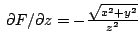
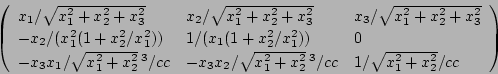
syms x y z
f1 = x^2+y^2 ; pdx1 = diff(f1,x); pdy1 = diff(f1,y)
%pdx1,pdy1  =   2*x  , 2*y
f2 = sin(x)*cos(y); pdx2 = diff(f2,x); pdy2 = diff(f2,y)
%pdx2,pdy2  =   cos(x)*cos(y);  -sin(x)*sin(y);
f3 = 1/sqrt(x^2+y^2+z^2); pdx3 = diff(f3,x);
pdy3 = diff(f3,y); pdz3 = diff(f3,y)y3 = diff(f3,y)
%pdx3, pdy3 =  -x/(sqrt(x^2+y^2+z^2))^3,  -y/(sqrt(x^2+y^2+z^2))^3
%   pdz3 =  -z/(sqrt(x^2+y^2+z^2))^3
60-12
%sincontgrad.m Konturplot mit eingezeichnetem Gradient
[X,Y] = meshgrid([0:.1:1]);
Z = sin(pi*X).*sin(pi*Y);
contour3(X,Y,Z,30)
figure(2); clf
[px,py] = gradient(Z,.2,.2);
contour(X,Y,Z)  ;  hold on
quiver(X,Y,px,py)             % malt Pfeile
axis equal ; hold off
60-13
%jhillcontgrad.m Konturplot mit eingezeichnetem Gradient
[X,Y] = meshgrid([-1600:50:1600],[-400:50:400]);
Z = max(1600 -(X/1000).^2*50 -(Y/250).^2*50,1400) ;
contour3(X,Y,Z,20); axis equal
figure(2); clf
[px,py] = gradient(Z,50,50);   %Abst\"ande zwischen Punkten
subplot(3,1,1)
contour(X,Y,Z,15)  ;  hold on
% Ausduennen der gezeichneten Pfeile
xsel = 1:4:65; ysel=1:2:17;
Xs = X(ysel,xsel);Ys = Y(ysel,xsel);
 pxs = px(ysel,xsel) ; pys = py(ysel,xsel);
quiver(Xs,Ys,pxs,pys)                % erstellt Pfeile
axis equal ;
subplot(3,1,2); contour(X,Y,px,15)
subplot(3,1,3); contour(X,Y,py,15)
 hold off
60-14 Die Funktions-M-Files können im allgemeinen Programm divfctcont() eingesetzt werden.
%z=minihillf(Xgr,Ygr) Funktion zur Definition der Flaeche
%    1 - x^2 - 0.2*y^2
function z=minihillf(Xgr,Ygr)
z = 1 - Xgr.^2 - 0.2*Ygr.^2 ;
%z=sinsinf(Xgr,Ygr) Funktion zur Definition der Flaeche
%    sin(pi*x) * sin(pi*y)
function z=sinsinf(Xgr,Ygr)
z = sin(pi*Xgr).*sin(pi*Ygr);
%z=pwdiff(Xgr,Ygr) Funktion zur Definition der Flaeche
%    (x^2 - abs(x^3)) *  (y^2 - abs(y^3))
function z=pwdiff(Xgr,Ygr)
z =(Xgr.^2 - abs(Xgr.^3)) .*  (Ygr.^2 - abs(Ygr.^3))  ;
function plhd = divfctcont(fctnam,xvec,yvec)
% plhd = divfctcont(fctnam,Xgrid,Ygrid)
%    Konturplot von mit 'fctnam' waehlbarer Funktion
[X,Y] = meshgrid(xvec,yvec);
Z = feval(fctnam,X,Y);
figure(1); clf
contour3(X,Y,Z,30)
figure(2); clf
[px,py] = gradient(Z,xvec,yvec);
plhd = contour(X,Y,Z,25)  ;  hold on
quiver(X,Y,px,py)                   %erstellt Pfeile
axis equal ; hold off
60-15
% p2p4findstat.m - Symbolic script sucht Stationaere Punkte
syms xs ys
fs = (xs^2-xs^4)*(ys^2-ys^4)
dfx = diff(fs,xs)
dfy = diff(fs,ys)
stptsol = solve(dfx,dfy)
stptsol.xs
stptsol.ys
%{xs 0} {0 ys}{+-1 +-1} {+-\sqrt(2)/2 +-\sqrt(2)/2}
%p2p4stat.m Konturplot mit stationaeren Punkten
[X,Y] = meshgrid([-1.1:0.1:1.1]);
Z = 10*(X.^2-X.^4).*(Y.^2-Y.^4) ;
figure(1); clf
contour3(X,Y,Z,20);
axis equal
figure(2); clf
contour(X,Y,Z,15)  ;
60-16 Mit der Funktion
%z=biquartf(Xgr,Ygr) Funktion zur Definition der Flaeche
%   0.25x^4-0.5x^2 + 0.25y^4-0.5y^2 -0.12x -0.05y + 1
function z=biquartf(Xgr,Ygr)
z=(0.25*Xgr.^4-0.5*Xgr.^2)-0.12*Xgr  ...
      +(0.25*Ygr.^4-0.5*Ygr.^2)+1-0.05*Ygr;
ergibt sich der Aufruf ganz einfach als:
divfctcont('biquartf',-1.7:0.2:1.7, -1.7:0.2:1.7)
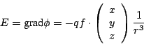
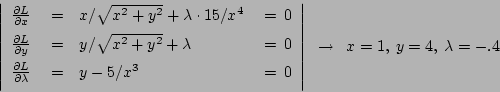
60-17 Die Funktion
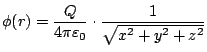 hat die drei partiellen Ableitungen
![]() damit ist
damit ist
60-18
x = 0:4 ; y = [1 1.2 2.2 3 3.6];
M1 = [sum(x.^2) sum(x); sum(x) 5]; b1 =[ sum(x.*y) ; sum(y)];
M2 = [sum(x.^4) sum(x.^3) sum(x.^2); sum(x.^3) sum(x.^2) sum(x); ...
       sum(x.^2) sum(x) 5];
b2 =[ sum(x.^2.*y) ; sum(x.*y) ; sum(y)];
M3 = [sum(x.^6) sum(x.^5) sum(x.^4) sum(x.^3);...
      sum(x.^5) sum(x.^4) sum(x.^3) sum(x.^2);
      sum(x.^4) sum(x.^3) sum(x.^2) sum(x);
      sum(x.^3) sum(x.^2) sum(x) 5 ];
b3 =[ sum(x.^3.*y); sum(x.^2.*y) ; sum(x.*y) ; sum(y)];
p1 = M1\b1
p2 = M2\b2
p3 = M3\b3
60-19
x = [-3 -2 -1 0 1 2 3]'; A=[x.^3 x.^2 x [1 1 1 1 1 1 1]'];
b = [-7 -5 -2 0 -1 2 0]'; p=A\b
60-20
x = (-2:2)' ; y = [-2 0 1 1.5 3]'; w = [4 2 1 2 4]';
Mn = [sum(x.^2) sum(x); sum(x) 5]; bn =[ sum(x.*y) ; sum(y)];
A = [x ones(5,1)];  pn = Mn\bn ; pf = A\y;
Aw = A.*[w w]; yw = y.*w;  pfw = Aw\yw;
Mw = [sum(w.^2.*x.^2) sum(x.*w.^2); sum(x.*w.^2) sum(w.^2)];
bw =[ sum(w.^2.*x.*y) ; sum(w.^2.*y)]; pnw = Mw\bw;
pn, pf, pnw, pfw
60-21 Mit Matrizen von 6-20: A'*A-Mn A'*y-bn Aw'*Aw-Mw Aw'*y-bw
60-22 Mit den Bibliotheksfunktionen:
x = (1:5)' ; y = [1 3 4 2 1]';
p2 = polyfit(x,y,2) ; p3 = polyfit(x,y,3)
xf = 0:0.05:6; y2 = polyval(p2,xf); y3 = polyval(p3,xf);
plot(x,y,'or'); hold on; plot(xf,y2); plot(xf,y3,'g')
60-23
x = (0:0.2:1)'*pi ; y = sin(x);
varfctfit(x,y,'pow0fct','pow1fct','pow2fct')

% pkoef = varfctfit(x,y,'f1','f2', ...)
%  linearer Fit nach einer variablen Anzahl Funktionen fk
function pkoef = varfctfit(varargin)
A=[];
for nf = 3:nargin
  A=[A feval(varargin{nf},varargin{1})];
end
pkoef = A\varargin{2};
60-24
x = (0:0.1:0.9)' ;
y = [0 1 1.2 0  1 0 0 0 0 -1]';
varfctfit(x,y,'sintpif')
varfctfit(x,y,'sintpif','sin2tpif')
varfctfit(x,y,'sintpif','sin2tpif','sin4tpif')
60-25
60-26
60-27
60-28
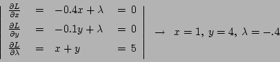
% hillagrange.m Figur zu Optimierung mit Nebenbedingung
xv = -6:0.1:6;
[xg,yg]=meshgrid(xv);
H =  10 - 0.02*xg.^2 - 0.1*yg.^2;
H = H .* (yg > xg-4) ; H=max(H,9);
figure(1) ; clf;  surf(xg,yg,H); view(15.5,11)
figure(2) ; clf
contour3(xg,yg,H)  ; hold on
LM = [-0.04 0 1 ; 0 -0.2 1 ; 1 -1 0]; Lb = [ 0 0 4]';
p= LM\Lb
xel = 0:0.1:6;  yel = -4+xel;
zel =  10 - 0.02*xel.^2 - 0.1*yel.^2;
zel = max(zel,9); plot3(xel,yel,zel,'k')
view(15.5,18.0) ; hold off
60-29
x=(-3:3)'; A=[x.^3 x.^2 x x.^0];
y1 = [-1 1 1 0 0 1 3]'; y2 = [1 2 1 2 3 3 5]';
% Aufruf der Singular Value Decomposition
[U , S , V] = svd(A);  Si = S
% nur S muss elementweise invertiert werden
for k=1:4
   Si(k,k) = 1/S(k,k);
end
Si
% U und V sind orthogonal: U'*U=I
Api= V*Si'*U';
p1 = A\y1
pp1 = Api*y1
p2 = A\y2
pp2 = Api*y2
60-30
![]()
60-31
x= [5 5]';  fct2p2p4iter;   fct2p2p4iter; fct2p2p4iter;
% fct2p2p4iter.m - run Jacobi-Iteration
fvec= fct2p2p4(x(1),x(2))
delx = fct2p2p4jac(x(1),x(2))\ fct2p2p4(x(1),x(2))
x = x-delx
% fvec = fct2p2p4(x,y) Funktion zur jacobi-Iteration
function fvec = fct2p2p4(x,y)
fvec = zeros(2,1);
fvec(1) = (x-4)^2+ y^2 -10;
fvec(2) = x^4+ y^4 -20;
%jac = fct2p2p4jac(x,y) Evaluation der Jacobi-Matrix
function jac = fct2p2p4jac(x,y)
jac = zeros(2);
jac(1,1) = 2*x-8;
jac(1,2) = 2*y;
jac(2,1) = 4*x^3;
jac(2,2) = 4*y^3;
60-32, 33 Siehe M-File-Sammlung.
T611 - Senkrecht zum Gradientenvektor, also
![]()
-
![]()
- Nur so wird die Nebenbedingung
als
![]() ein Teil des Gleichungssystems.
ein Teil des Gleichungssystems.
-
![]()
T612
[X,Y]=meshgrid(-1:0.02:1); h=max(1-X.^2-Y.^2,0); h=h.^2;
contour3(X,Y,h,25); axis equal
T613
hA=0; hB=1; hC=4; hD=1; [X,Y]=meshgrid(0:0.1:5);
h=hA + (hB-hA)*X/5 + (hD-hA)*Y/5 + (hC+hA-hD-hB)*Y.*X/25;
contour3(X,Y,h,25); axis equal; box on; pause
[gx,gy] = gradient(h,0.1,0.1); contour(X,Y,gx); pause
contour(X,Y,gy);
T614
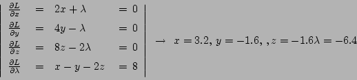
![\begin{displaymath}
\left\vert
\begin{array}{lclc}
\frac{\partial L}{\partial x...
...}
& ~=~& x+2y+4z -8
& ~=~ 0\\ [0.5em]
\end{array}\right\vert
\end{displaymath}](img729.png)
M=[8 0 0 1; 0 2 0 0; 0 0 0 4; 1 2 4 0]; b=[0 0 -1 8];
x = [0.312 0.25 1.8672 -0.25]'
T615
% newtexa als Funtion damit f und jac intern sind
function xf = newtexa(xi,yi)
xv=[xi;yi];
for k=1:8; xv = xv-newtexajac(xv)\newtexafct(xv); end;
xf=xv;
% fvec = newtexafct(xv) Beispielfunktion 2D Newton
function fvec = newtexafct(xv)
fvec = zeros(2,1); fvec(1) = xv(1)^4+xv(2)^4-20;
fvec(2) = xv(1)^2 -xv(2)^2 -1;
%  newtexajac(xv) Beispielfunktion jac zu 2D Newton
function jac = newtexajac(xv)
jac(1,1)=4*xv(1)^3 ; jac(1,2)=4*xv(2)^3 ;
jac(2,1)=2*xv(1) ; jac(2,2)=-2*xv(2) ;